SINDy-SHRED Tutorial on Sea Surface Temperature#

Import Libraries#

# PYSHRED
from pyshred import DataManager, SHRED, SHREDEngine, SINDy_Forecaster

# Other helper libraries
import matplotlib.pyplot as plt
from scipy.io import loadmat
import torch
import numpy as np

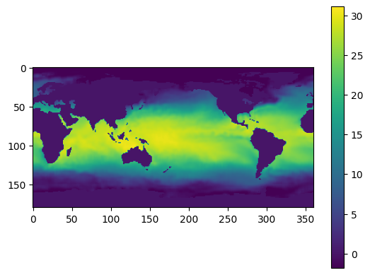
Load in SST Data#

sst_data = np.load("sst_data.npy")

# Plotting a single frame
plt.figure()
plt.imshow(sst_data[0]) 
plt.colorbar()
plt.show()

png

Initialize Data Manager#

manager = DataManager(
    lags = 52,
    train_size = 0.8,
    val_size = 0.1,
    test_size = 0.1,
)

Add datasets and sensors#

manager.add_data(
    data = sst_data,
    id = "SST",
    random = 50,
    # mobile=,
    # stationary=,
    # measurements=,
    compress=False,
)

Analyze sensor summary#

manager.sensor_summary_df

	data id	sensor_number	type	loc/traj
0	SST	0	stationary (random)	(40, 343)
1	SST	1	stationary (random)	(136, 255)
2	SST	2	stationary (random)	(66, 219)
3	SST	3	stationary (random)	(75, 5)
4	SST	4	stationary (random)	(2, 206)
5	SST	5	stationary (random)	(43, 229)
6	SST	6	stationary (random)	(121, 31)
7	SST	7	stationary (random)	(46, 136)
8	SST	8	stationary (random)	(43, 88)
9	SST	9	stationary (random)	(147, 153)
10	SST	10	stationary (random)	(105, 14)
11	SST	11	stationary (random)	(154, 16)
12	SST	12	stationary (random)	(142, 151)
13	SST	13	stationary (random)	(144, 320)
14	SST	14	stationary (random)	(171, 86)
15	SST	15	stationary (random)	(55, 318)
16	SST	16	stationary (random)	(154, 84)
17	SST	17	stationary (random)	(45, 16)
18	SST	18	stationary (random)	(142, 319)
19	SST	19	stationary (random)	(145, 241)
20	SST	20	stationary (random)	(82, 164)
21	SST	21	stationary (random)	(54, 195)
22	SST	22	stationary (random)	(105, 310)
23	SST	23	stationary (random)	(178, 123)
24	SST	24	stationary (random)	(112, 242)
25	SST	25	stationary (random)	(139, 358)
26	SST	26	stationary (random)	(149, 227)
27	SST	27	stationary (random)	(10, 98)
28	SST	28	stationary (random)	(109, 97)
29	SST	29	stationary (random)	(38, 245)
30	SST	30	stationary (random)	(97, 217)
31	SST	31	stationary (random)	(104, 23)
32	SST	32	stationary (random)	(155, 71)
33	SST	33	stationary (random)	(134, 41)
34	SST	34	stationary (random)	(66, 215)
35	SST	35	stationary (random)	(173, 194)
36	SST	36	stationary (random)	(172, 139)
37	SST	37	stationary (random)	(57, 337)
38	SST	38	stationary (random)	(56, 298)
39	SST	39	stationary (random)	(125, 245)
40	SST	40	stationary (random)	(160, 347)
41	SST	41	stationary (random)	(166, 283)
42	SST	42	stationary (random)	(85, 26)
43	SST	43	stationary (random)	(62, 346)
44	SST	44	stationary (random)	(96, 65)
45	SST	45	stationary (random)	(121, 335)
46	SST	46	stationary (random)	(128, 251)
47	SST	47	stationary (random)	(122, 62)
48	SST	48	stationary (random)	(96, 69)
49	SST	49	stationary (random)	(73, 237)

manager.sensor_measurements_df

	SST-0	SST-1	SST-2	SST-3	SST-4	SST-5	SST-6	SST-7	SST-8	SST-9	...	SST-40	SST-41	SST-42	SST-43	SST-44	SST-45	SST-46	SST-47	SST-48	SST-49
0	11.74	10.08	22.190000	0.0	-1.80	11.12	25.069999	2.78	0.0	3.28	...	0.15	-0.0	0.0	20.200000	29.159999	22.689999	15.22	21.740000	28.719999	24.539999
1	11.67	10.21	22.100000	0.0	-1.80	10.70	24.049999	2.12	0.0	3.61	...	0.06	-0.0	0.0	19.910000	28.129999	23.609999	14.96	22.589999	28.189999	24.279999
2	11.73	10.61	21.890000	0.0	-1.80	10.29	24.849999	1.53	0.0	3.63	...	0.31	-0.0	0.0	19.170000	28.789999	23.079999	15.90	21.410000	28.639999	24.899999
3	11.33	10.91	21.600000	0.0	-1.80	9.87	24.879999	1.68	0.0	3.72	...	0.53	-0.0	0.0	19.180000	28.539999	23.349999	17.87	22.350000	28.559999	24.389999
4	11.17	11.19	21.590000	0.0	-1.80	9.45	24.889999	1.35	0.0	3.76	...	0.52	-0.0	0.0	18.770000	28.059999	23.999999	17.69	22.100000	28.449999	24.219999
...	...	...	...	...	...	...	...	...	...	...	...	...	...	...	...	...	...	...	...	...	...
1395	15.89	8.09	24.459999	0.0	-1.70	17.31	21.770000	17.67	0.0	1.56	...	-1.75	-0.0	0.0	21.540000	27.819999	18.070000	11.61	16.390000	27.649999	27.269999
1396	15.61	8.22	24.159999	0.0	-1.78	16.82	20.870000	16.34	0.0	1.83	...	-1.70	-0.0	0.0	21.690000	28.039999	17.930000	11.92	16.970000	27.649999	26.809999
1397	15.17	8.34	24.369999	0.0	-1.80	16.12	20.980000	14.77	0.0	1.41	...	-1.65	-0.0	0.0	21.740000	28.209999	17.940000	12.23	17.360000	27.799999	26.839999
1398	14.79	8.75	24.199999	0.0	-1.80	15.60	21.330000	13.03	0.0	1.87	...	-1.47	-0.0	0.0	21.840000	28.019999	18.140000	12.83	17.410000	27.619999	26.679999
1399	14.71	8.75	24.239999	0.0	-1.80	14.83	21.560000	11.23	0.0	2.12	...	-1.32	-0.0	0.0	22.449999	28.499999	18.500000	12.71	17.740000	28.489999	26.969999

1400 rows × 50 columns

Get train, validation, and test set#

train_dataset, val_dataset, test_dataset= manager.prepare()

Initialize a latent forecaster#

latent_forecaster = SINDy_Forecaster(poly_order=1, include_sine=True, dt=1/5)

Initialize SHRED#

shred = SHRED(sequence_model="GRU", decoder_model="MLP", latent_forecaster=latent_forecaster)

Fit SHRED#

val_errors = shred.fit(train_dataset=train_dataset, val_dataset=val_dataset, num_epochs=10, sindy_thres_epoch=20, sindy_regularization=1)
print('val_errors:', val_errors)

Fitting SindySHRED...
Epoch 1: Average training loss = 0.091680
Validation MSE (epoch 1): 0.032684
Epoch 2: Average training loss = 0.032257
Validation MSE (epoch 2): 0.015280
Epoch 3: Average training loss = 0.020602
Validation MSE (epoch 3): 0.013595
Epoch 4: Average training loss = 0.018892
Validation MSE (epoch 4): 0.013358
Epoch 5: Average training loss = 0.017929
Validation MSE (epoch 5): 0.013441
Epoch 6: Average training loss = 0.017431
Validation MSE (epoch 6): 0.013291
Epoch 7: Average training loss = 0.017039
Validation MSE (epoch 7): 0.014045
Epoch 8: Average training loss = 0.016548
Validation MSE (epoch 8): 0.013414
Epoch 9: Average training loss = 0.015898
Validation MSE (epoch 9): 0.013693
Epoch 10: Average training loss = 0.015332
Validation MSE (epoch 10): 0.013768
val_errors: [0.03268439 0.01527982 0.01359512 0.01335787 0.01344112 0.01329135
 0.01404459 0.01341446 0.0136935  0.01376815]

Evaluate SHRED#

train_mse = shred.evaluate(dataset=train_dataset)
val_mse = shred.evaluate(dataset=val_dataset)
test_mse = shred.evaluate(dataset=test_dataset)
print(f"Train MSE: {train_mse:.3f}")
print(f"Val   MSE: {val_mse:.3f}")
print(f"Test  MSE: {test_mse:.3f}")

Train MSE: 0.010
Val   MSE: 0.014
Test  MSE: 0.018

SINDy Discovered Latent Dynamics#

print(shred.latent_forecaster)

(x0)' = 0.269 1 + 0.326 x0 + -0.079 x1 + 0.486 x2
(x1)' = 0.449 1 + 0.333 x0 + -0.308 x1 + 0.189 x2
(x2)' = -0.492 1 + -0.529 x0 + 0.191 x1 + -0.292 x2

Initialize SHRED Engine for Downstream Tasks#

engine = SHREDEngine(manager, shred)

Sensor Measurements to Latent Space#

test_latent_from_sensors = engine.sensor_to_latent(manager.test_sensor_measurements)

Forecast Latent Space (No Sensor Measurements)#

val_latents = engine.sensor_to_latent(manager.val_sensor_measurements)
init_latents = val_latents[-1] # seed forecaster with final latent space from val
h = len(manager.test_sensor_measurements)
test_latent_from_forecaster = engine.forecast_latent(h=h, init_latents=init_latents)

Decode Latent Space to Full-State Space#

test_prediction = engine.decode(test_latent_from_sensors) # latent space generated from sensor data
test_forecast = engine.decode(test_latent_from_forecaster) # latent space generated from latent forecasted (no sensor data)

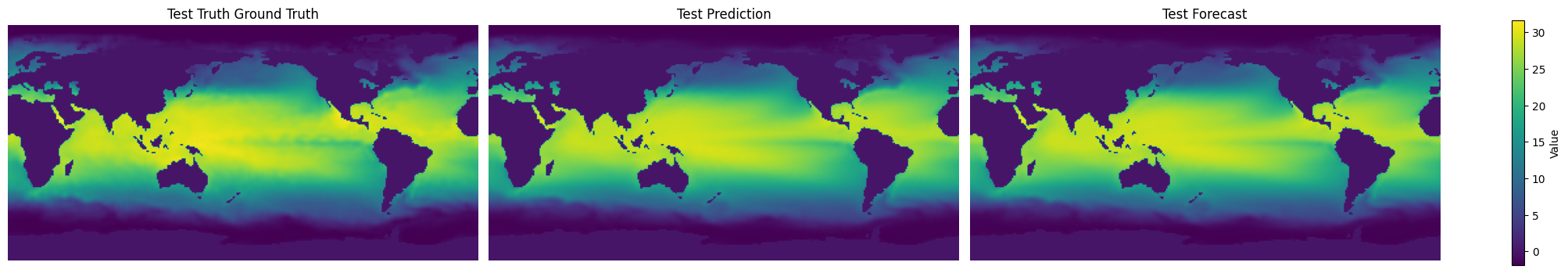
Compare final frame in prediction and forecast to ground truth:

truth      = sst_data[-1]
prediction = test_prediction['SST'][-1]
forecast   = test_forecast['SST'][-1]

data   = [truth, prediction, forecast]
titles = ["Test Truth Ground Truth", "Test Prediction", "Test Forecast"]

vmin, vmax = np.min([d.min() for d in data]), np.max([d.max() for d in data])

fig, axes = plt.subplots(1, 3, figsize=(20, 4), constrained_layout=True)

for ax, d, title in zip(axes, data, titles):
    im = ax.imshow(d, vmin=vmin, vmax=vmax)
    ax.set(title=title)
    ax.axis("off")

fig.colorbar(im, ax=axes, label="Value", shrink=0.8)

<matplotlib.colorbar.Colorbar at 0x250fe875750>

png

Evaluate MSE on Ground Truth Data#

# Train
t_train = len(manager.train_sensor_measurements)
train_Y = {'SST': sst_data[0:t_train]}
train_error = engine.evaluate(manager.train_sensor_measurements, train_Y)

# Val
t_val = len(manager.test_sensor_measurements)
val_Y = {'SST': sst_data[t_train:t_train+t_val]}
val_error = engine.evaluate(manager.val_sensor_measurements, val_Y)

# Test
t_test = len(manager.test_sensor_measurements)
test_Y = {'SST': sst_data[-t_test:]}
test_error = engine.evaluate(manager.test_sensor_measurements, test_Y)

print('---------- TRAIN ----------')
print(train_error)
print('\n---------- VAL   ----------')
print(val_error)
print('\n---------- TEST  ----------')
print(test_error)

---------- TRAIN ----------
              MSE      RMSE       MAE        R2
dataset                                        
SST      0.580466  0.761883  0.425608  0.407465

---------- VAL   ----------
              MSE     RMSE       MAE        R2
dataset                                       
SST      0.936849  0.96791  0.498381 -0.579918

---------- TEST  ----------
              MSE      RMSE       MAE        R2
dataset                                        
SST      1.248095  1.117182  0.587646 -0.453009