SHRED-ROM Tutorial on Kuramoto Sivashinsky#

Import Libraries#

# PYSHRED
import pyshred
from pyshred import ParametricDataManager, SHRED, ParametricSHREDEngine

# Other helper libraries
import matplotlib.pyplot as plt
from scipy.io import loadmat
import torch
import numpy as np

The autoreload extension is already loaded. To reload it, use:
  %reload_ext autoreload

Load Kuramoto Sivashinsky dataset#

import numpy as np
import urllib.request
# URL of the NPZ file
url = 'https://zenodo.org/records/14524524/files/KuramotoSivashinsky_data.npz?download=1'
# Local filename to save the downloaded file
filename = 'KuramotoSivashinsky_data.npz'
# Download the file from the URL
urllib.request.urlretrieve(url, filename)
# Load the data from the NPZ file
dataset = np.load(filename)

Device Info#

device = pyshred.set_device("auto")
# device = pyshred.set_device("cpu") # force CPU
# device = pyshred.set_device("cuda") # force CUDA
# device = pyshred.set_device("mps") # force MPS
# device = pyshred.set_device("cuda", device_id=0) # force specific GPU
pyshred.device_info()

=== PyShred Device Information ===
Current device: cpu
Device config: DeviceConfig(device_type=<DeviceType.AUTO: 'auto'>, device_id=None, force_cpu=False, warn_on_fallback=True)

Device Availability:
  CUDA available: False
  MPS available: False
  CPU: Always available

Initialize Data Manager#

# Initialize ParametricSHREDDataManager
manager = ParametricDataManager(
    lags = 20,
    train_size = 0.8,
    val_size = 0.1,
    test_size = 0.1,
    )

Add datasets and sensors#

data = dataset['u'] # shape (500, 201, 100)
params = dataset['mu'] # shape (500, 201, 2)


manager.add_data(
    data=data,
    random=3,
    # stationary=[(15,),(30,),(45,)],
    id = 'KS',
    compress = False
)

# add params
manager.add_data(
    data=params,
    # stationary=[(15,),(30,),(45,)],
    id = 'MU',
    compress = False
)

Analyze sensor summary#

manager.sensor_measurements_df

	KS-0	KS-1	KS-2
0	-0.434038	-1.148071	0.154032
1	-0.457136	-0.961066	0.332515
2	-0.459894	-0.912785	0.361393
3	-0.446475	-0.873385	0.404951
4	-0.389743	-0.829674	0.485893
...	...	...	...
100495	-0.846195	-1.008426	0.261712
100496	-1.671882	-0.458563	-0.622521
100497	-2.103602	0.638096	-1.591052
100498	-1.971333	1.887684	-2.129965
100499	-1.450100	2.538589	-2.005693

100500 rows × 3 columns

manager.sensor_summary_df

	data id	sensor_number	type	loc/traj
0	KS	0	stationary (random)	(18,)
1	KS	1	stationary (random)	(93,)
2	KS	2	stationary (random)	(15,)

Get train, validation, and test set#

train_dataset, val_dataset, test_dataset= manager.prepare()

Initialize SHRED#

When using a ParametricDataManager, ensure latent_forecaster is set to None.

shred = SHRED(sequence_model="LSTM", decoder_model="MLP", latent_forecaster=None)

Fit SHRED#

val_errors = shred.fit(train_dataset=train_dataset, val_dataset=val_dataset, num_epochs=20, sindy_regularization=0)
print('val_errors:', val_errors)

Fitting SHRED...
Epoch 1: Average training loss = 0.031690
Validation MSE (epoch 1): 0.026569
Epoch 2: Average training loss = 0.016993
Validation MSE (epoch 2): 0.015352
Epoch 3: Average training loss = 0.011736
Validation MSE (epoch 3): 0.012691
Epoch 4: Average training loss = 0.009915
Validation MSE (epoch 4): 0.011286
Epoch 5: Average training loss = 0.008901
Validation MSE (epoch 5): 0.010464
Epoch 6: Average training loss = 0.008259
Validation MSE (epoch 6): 0.009664
Epoch 7: Average training loss = 0.007670
Validation MSE (epoch 7): 0.008933
Epoch 8: Average training loss = 0.007126
Validation MSE (epoch 8): 0.008480
Epoch 9: Average training loss = 0.006610
Validation MSE (epoch 9): 0.008143
Epoch 10: Average training loss = 0.006278
Validation MSE (epoch 10): 0.008485
Epoch 11: Average training loss = 0.005930
Validation MSE (epoch 11): 0.007433
Epoch 12: Average training loss = 0.005582
Validation MSE (epoch 12): 0.006999
Epoch 13: Average training loss = 0.005281
Validation MSE (epoch 13): 0.006656
Epoch 14: Average training loss = 0.005139
Validation MSE (epoch 14): 0.006386
Epoch 15: Average training loss = 0.004810
Validation MSE (epoch 15): 0.005950
Epoch 16: Average training loss = 0.004614
Validation MSE (epoch 16): 0.005578
Epoch 17: Average training loss = 0.004570
Validation MSE (epoch 17): 0.005578
Epoch 18: Average training loss = 0.004257
Validation MSE (epoch 18): 0.005292
Epoch 19: Average training loss = 0.004113
Validation MSE (epoch 19): 0.005244
Epoch 20: Average training loss = 0.004088
Validation MSE (epoch 20): 0.005059
val_errors: [0.02656859 0.0153518  0.01269077 0.01128609 0.01046397 0.00966403
 0.00893335 0.00848005 0.00814289 0.00848533 0.00743333 0.00699905
 0.00665622 0.00638625 0.00594996 0.00557757 0.00557818 0.00529238
 0.00524372 0.00505928]

Evaluate SHRED#

train_mse = shred.evaluate(dataset=train_dataset)
val_mse = shred.evaluate(dataset=val_dataset)
test_mse = shred.evaluate(dataset=test_dataset)
print(f"Train MSE: {train_mse:.3f}")
print(f"Val   MSE: {val_mse:.3f}")
print(f"Test  MSE: {test_mse:.3f}")

Train MSE: 0.003
Val   MSE: 0.005
Test  MSE: 0.004

Initialize Parametric SHRED Engine for Downstream Tasks#

engine = ParametricSHREDEngine(manager, shred)

Sensor Measurements to Latent Space#

test_latent_from_sensors = engine.sensor_to_latent(manager.test_sensor_measurements)

Decode Latent Space to Full-State Space#

test_prediction = engine.decode(test_latent_from_sensors) # latent space generated from sensor data

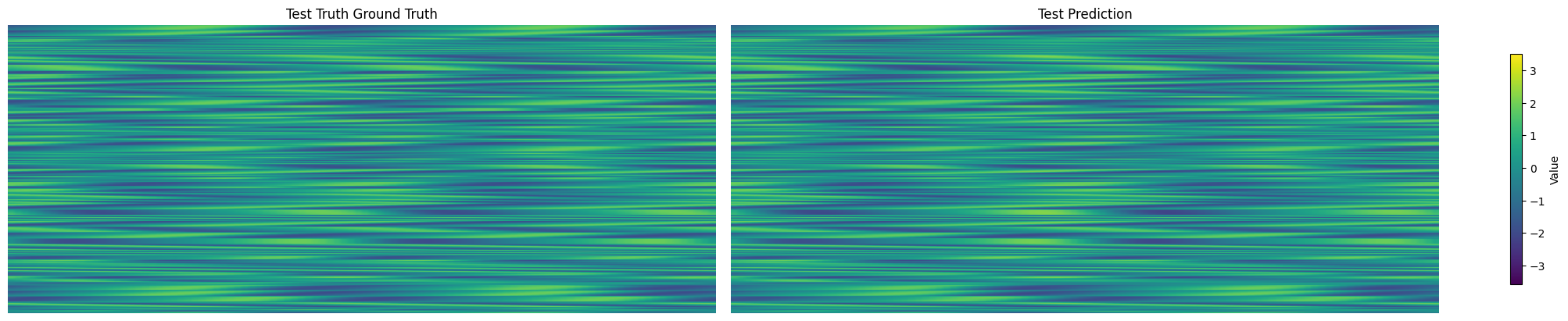
Compare prediction against the truth#

Since both number of trajectories (data.shape[0]) and number of timesteps (data.shape[1]) are both variable, we will leave them combined on the first axis. The remaining axes are all spatial dimensions.

spatial_shape = data.shape[2:]
test_data = data[manager.test_indices]
truth      = test_data.reshape(-1, *spatial_shape)
prediction = test_prediction['KS']

compare_data = [truth, prediction]
titles = ["Test Truth Ground Truth", "Test Prediction"]

vmin, vmax = np.min([d.min() for d in compare_data]), np.max([d.max() for d in compare_data])

fig, axes = plt.subplots(1, 2, figsize=(20, 4), constrained_layout=True)

for ax, d, title in zip(axes, compare_data, titles):
    im = ax.imshow(d, vmin=vmin, vmax=vmax, aspect='auto')
    ax.set(title=title)
    ax.axis("off")

fig.colorbar(im, ax=axes, label="Value", shrink=0.8)

<matplotlib.colorbar.Colorbar at 0x2a69c042da0>

png

Predicted params#

params_prediction = test_prediction['MU']
print(params_prediction.shape)
params_prediction

(10050, 2)





array([[1.502923 , 2.701217 ],
       [1.5866294, 4.104658 ],
       [1.6049353, 4.049966 ],
       ...,
       [1.0774401, 2.5793262],
       [0.9692009, 2.925611 ],
       [1.0723687, 2.6876066]], dtype=float32)

Evaluate MSE on Ground Truth Data#

Since both number of trajectories (data.shape[0]) and number of timesteps (data.shape[1]) are both variable, we will leave them combined on the first axis. The remaining axes are all spatial dimensions.

# Train
t_train = len(manager.train_sensor_measurements)
train_Y = {'KS': data[0:t_train].reshape(-1, *spatial_shape)} # unpack the spatial dimensions
train_error = engine.evaluate(manager.train_sensor_measurements, train_Y)

# Val
t_val = len(manager.test_sensor_measurements)
val_Y = {'KS': data[t_train:t_train+t_val].reshape(-1, *spatial_shape)}
val_error = engine.evaluate(manager.val_sensor_measurements, val_Y)

# Test
t_test = len(manager.test_sensor_measurements)
test_Y = {'KS': data[-t_test:].reshape(-1, *spatial_shape)}
test_error = engine.evaluate(manager.test_sensor_measurements, test_Y)

print('---------- TRAIN ----------')
print(train_error)
print('\n---------- VAL   ----------')
print(val_error)
print('\n---------- TEST  ----------')
print(test_error)

---------- TRAIN ----------
              MSE      RMSE       MAE        R2
dataset                                        
KS       0.085787  0.292894  0.189655  0.934717

---------- VAL   ----------
            MSE      RMSE       MAE        R2
dataset                                      
KS       0.1452  0.381051  0.237308  0.887799

---------- TEST  ----------
             MSE     RMSE       MAE        R2
dataset                                      
KS       0.08774  0.29621  0.185969  0.933305